/Project Details
Applied Bayesian Analysis of World Happiness
Built Bayesian regression and hierarchical models with brms to explain country-level happiness using GDP, social support, health, and regional structure.

This Applied Bayesian Analysis project focuses on modeling country-level happiness scores using the World Happiness Report 2024 dataset. The main predictors are GDP, social support, and healthy life expectancy, while continent and region information is used to define the hierarchical structure.
The analysis was implemented in R with brms, the Bayesian regression modeling package developed by Prof. Dr. Paul Bürkner. This places the project directly inside a modern Bayesian workflow built around expressive model formulas, Stan-backed sampling, posterior checks, and uncertainty-aware interpretation.
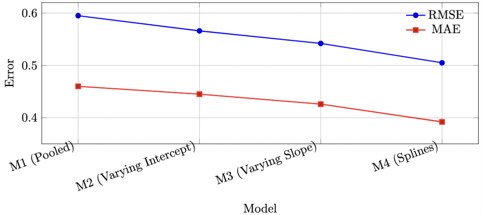
The workflow starts with data cleaning, missing-value handling, correlation checks, region mapping, and exploratory visualization. From there, I fit four models in sequence: a pooled Gaussian regression, a varying-intercept model by region, a varying-slope model for GDP by region, and a spline-based model for non-linear health effects.
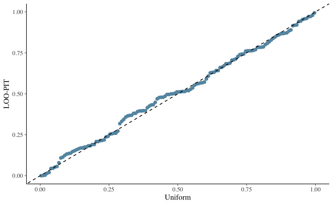
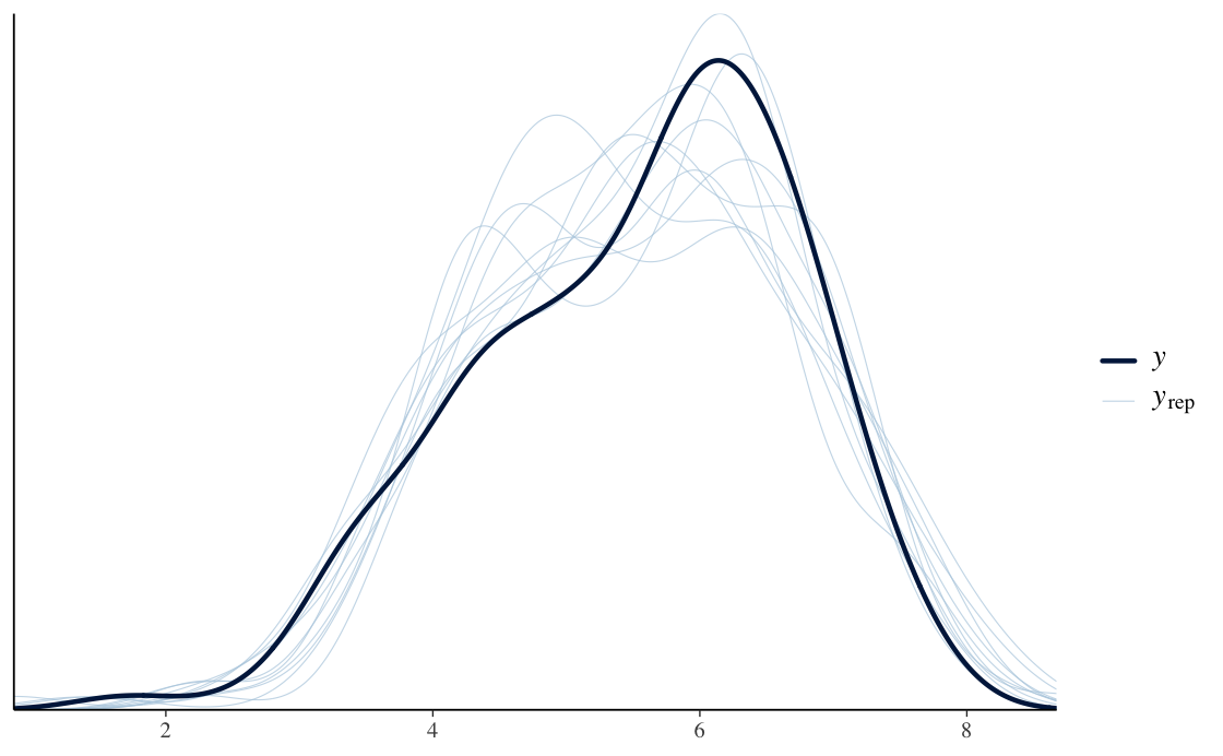
A central part of the project was not only fitting the models, but checking them carefully. I compared model behavior and predictive quality using trace plots, posterior summaries, posterior predictive checks, conditional effects, LOO-PIT style checks, Bayesian R2, RMSE, and MAE.
Highlights
- Cleaned World Happiness Report 2024 data from 143 to 140 complete country observations.
- Mapped countries into regions to support hierarchical Bayesian modeling.
- Fit pooled, varying-intercept, varying-slope, and spline-based models using brms and Stan.
- Used weakly informative priors such as normal priors for coefficients and exponential priors for group-level standard deviations.
- Evaluated models with posterior predictive checks, trace diagnostics, conditional effects, Bayesian R2, RMSE, and MAE.
- Framed uncertainty as a first-class output rather than hiding it behind a single point estimate.
Model Formulas
y_i ~ Normal(β0 + β1 * GDP_i + β2 * Support_i + β3 * Health_i, σ) Baseline Gaussian regression with shared coefficients across all countries.
y_i ~ Normal(α_region[i] + β1 * GDP_i + β2 * Support_i + β3 * Health_i, σ), α_r ~ Normal(μ_α, τ_α) Allows each region to have its own baseline happiness level.
y_i ~ Normal(α_region[i] + β1,region[i] * GDP_i + β2 * Support_i + β3 * Health_i, σ), β1,r ~ Normal(μ_β1, τ_β1) Lets the GDP effect vary across regions while keeping the remaining effects fixed.
y_i ~ Normal(α_region[i] + β1,region[i] * GDP_i + β2 * Support_i + s(Health_i), σ) Extends the hierarchical setup with a smooth non-linear effect for health.
Figures